A Primer on Financial Derivatives

August 20, 2019

Financial derivatives are used for commodities, like corn, oil, gasoline, or gold, and for currencies, like the U.S. Dollar and the Euro. However, there are derivatives based on stocks, bonds, interest rates, and indices. Companies use derivatives to lower their operational risk for the delivery of raw materials and the changes in exchange rates or in interest rates. Trading requires a small down payment (margin) and usually consists of rolling positions (contracts are liquidated by another derivative before coming to term).

Market Assumptions

The market is assumed to contain many buyers and sellers (liquidity), the information about the details of a contract are publicly and uniformly available to buyers and sellers, and the market is completely regulated and balanced by the forces of supply and demand (competition). Thus, in such an efficient market with no chances of arbitrage, any contract will be priced at a fair price just by the forces of supply and demand. Specifically, a contract with N cash flows can be priced using present value and no-arbitrage by replicating (lower bound ) and reversing (upper bound) its cash flows by borrowing and lending at interest rates corresponding to the discount rate of the PV. If borrowing and lending rates are the same the bounds overlap and the price is one, otherwise is a range.

Market Risks

Risks influencing equity financial derivatives include: price risk (uncertainty in the underlying’s price change), volatility risk (the standard deviation of the underlying’s returns), stochastic jump or crash risk, interest rate risk (via risk-neutral discounting with the short rate), correlation risk (higher among asset classes during times of stress), liquidity risk (if certain options are not liquidly traded the desired hedge may not be executable), default risk (default of the underlying).

Statistical Properties of Stocks and Stocks’ Indices

In general, the following set of statistical properties, common across many instruments, markets and time periods, has been observed by independent studies:

stochastic volatility: volatility changes in an unpredictable manner, it is neither constant nor deterministic
volatility clustering: high volatility events usually cluster in time resulting in a positive autocorrelation of volatility metrics
volatility mean reversion: volatility oscillates around its changing mean
leverage effect: volatility is negatively correlated with asset returns; if return measures increase, volatility measures often decrease and vice versa
fat tails: with respect to a normal distribution large positive and negative index returns are more frequent
jumps: levels may move by magnitudes not explained with Gaussian diffusion; thus, a jump component is required to explain some large moves

Floating interests and Terms Structure

Computing the price of a floating rate bond by discounting its cash flows at the future rate results in an expression containing a random quantity. However, computing the price by using the arbitrage-free and replication argument will result in deterministic cash flows because the face value of the bond simplifies with the random part of the cash flow. Indeed, the arbitrage-free price of a floating rate bond is equal to its face value. Spot rates are the rates used in the discount factors corresponding to the maturity of the loans; thus, it is possible to infer spot rates from bond prices. Forward rates are interest rates quoted today for lending in the future. Spot rates and forward rates are algebraically related. Interest rates depend on the term or duration of the loan: investors prefer their funds to be liquid rather than tied up and have to be offered a higher rate to lock in funds for a longer period. Interest rates depend also on expectations of future rates and market segmentation.

Statistical Properties of Short Rates

Short rates are relevant parameters of all asset pricing models; specifically, the most important statistical properties for financial modeling are:

positivity: nominal interest rates are positive in general
stochasticity: interest rates in general and short rates in particular move in a random and unpredictable manner
mean reversion: interest rates can neither trend to zero nor infinity in the long term such that there must always be the phenomenon of mean reversion
term structure: yields of benchmark bonds—like German bunds—as well as rates in interbank lending vary with time to maturity implying different (instantaneous) forward rates implying different future short rate levels

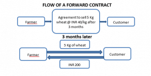
Forward Contracts

A forward contract gives the buyer the right and the obligation to purchase a specified amount of an asset at a specified time T at a specified price F (the forward price) set at time t = 0. Example contracts include:

Delivery of stock with maturity 6 months
Sale of gold with maturity 1 year
Buy 10m $ worth of Euros with maturity 3 months
Delivery of 9-month T-Bill with maturity 3 months

The collateral future price (forward price) is defined using the no-arbitrage and replicating arguments in order to elide the random quantity in the replicating cash flow by assuming the collateral future price specified in the forward at time zero equals the collateral spot price at expiration time T discounted by the spot interest rate with the term corresponding to the forward maturity. Instead, the value of the contract at any time t is given by the difference of the underlying value between time t and maturity (difference of the forward price of the asset) discounted back from maturity T to time t using a corresponding forward rate.

Swap

A more common instrument among financial derivatives is the swap. A swap is an agreement between two parties to exchange a series of future cash flows. For most types of swaps, one party makes payments that are determined by a random outcome, such as an interest rate, a currency rate, an equity return, or a commodity price. These payments are commonly referred to as variable or floating. The other party either makes floating payments determined by some other random factor or makes fixed payments. When a swap is initiated, neither party pays any amount to the other: a swap has zero value at the start of the contract. Each date on which the parties make payments is called a settlement date, and the time between settlement dates is called the settlement period. Both sets of payments are made in the same currency, consequently, the parties typically agree to exchange only the net amount owed from one party to the other, a practice called netting. A plain vanilla swap is simply an interest rate swap in which one party pays a fixed rate and the other pays a floating rate, with both sets of payments in the same currency. Again, by using replicating and no-arbitrage arguments the random part of the cashflow is eliminated assuming a periodic fixed interest rate X such that the value of the swap is nothing. Note that the annual rate is obtained multiplying X by the number of periods in one year, depending on the term structure considered. Thus, the value of the swap is given by the difference in basis point between X and the floating rate times the notional.

Futures

Futures are financial derivatives absolving an important function in markets. Because forwards are not organized through an exchange, they do not provide price transparency and unique pricing. Futures contract solve the problem of a multitude of prices for the same maturity by marking-to-market (computing profits/losses day by day, on account). Futures are organized on OTC exchanges and can be written on any underlying security with a settlement price: commodities, S&P500, Russel 2000, VIX. Futures contracts are standardized and have high leverage and liquidity, but clearly more risk and less flexibility because only linear payoffs can be hedged (futures prices are an approximately linear function of the underlying). The cash flow pattern from the viewpoint of a buyer or seller of a futures contract is different from and more complex than the cash flow pattern from a forward contract. At the close of each trading day, the gain or loss from the price change that occurred over that day is immediately credited or debited to the accounts of the individuals who are long or short. Furthermore, all contracts are rewritten so that the price at which parties are obliged to buy and sell the financial instrument is the price of the future at the close of the day. The aggregate profit or loss from the contract over its life would be the same whether it is a forward or a futures contract, but the timing of the cash flows is obviously very different.

As the futures contract approaches expiration, the spot price/market price and the futures price converge and both are equal at contract expiration. The more in the money a contract is the higher its futures contract value; the closer the expiration, the higher the volume trading. In general, a roll option allows extending the contract at a new price for a new expiration; roll yield is the (positive/negative) return generated by rolling a short-term futures contract into a longer-term. When the Spot Price of the underlying is lesser than the Futures Price at a particular point in time (for a specific contract and date), the situation is called Contango. The market is said to be in Contango whenever all the contracts’ futures prices are higher than the day’s spot price (upward sloping curve). Normal contango refers to a market usually experiencing contango. An initial long futures position experiencing Contango leads to a negative roll-yield. Backwardation is just the opposite case. The two effects depend on excessive demand or oversupply either for spot asset or futures. Additionally, Contango is a function of the rising cost of carrying the underlying lowering the spot and increasing the future price cost; (higher) interest rates have a similar effect. Instead, Backwardation can also be driven by the convenience yield occurring whenever a shortage in the underlying drive down the future and up the spot.

Options

The most common contract among financial derivatives is the option. An option is a contract entitling the holder to buy or sell designated security at or within a certain period of time at a particular price. Options contracts are characterized by a nonlinear payoff because the price depends on a nonlinear function of the underlying. Thus, it is impossible to price without a model for the underlying but the assumptions of mathematical finance (not moving the market; liquidity, jumps; shorting; fractional quantities; no transaction costs) substantially make difficult to determine a single model always valid with the changing market conditions. The simplest of the option pricing formulas is the binomial option pricing formula which input variables are easily observed, except for one—the variance of the instantaneous rate of return on the stock. Such a value can be inferred from historical data but also through the Black–Scholes formula. Assuming option prices are such that the Black–Scholes model holds on average, then the market price of the option can be substituted in the model to obtain the instantaneous rate of the variance of the stock.

Volatility and its Statistical Properties

In general, it does not exist a single definition or concept of volatility but rather a family of definitions related to the notion of an undirected dispersion/risk measure:

historical volatility refers to the standard deviation of log-returns of a financial time series
instantaneous volatility refers to the volatility factor of a diffusion process; for example, in the Black- Scholes-Merton model the instantaneous volatility σ is found in the respective (risk-neutral) stochastic differential equation (SDE)
implied volatility is the volatility that, if put into the Black-Scholes-Merton option pricing formula, gives the market-observed price of an option

The volatility surface for options has the following statistical properties:

smiles: option implied volatilities exhibit a smile form (slightly U shaped); this is a phenomenon present since the market crash of 1987
term structure: smiles are more pronounced for short-term options than for longer-term options; a phenomenon sometimes called volatility term structure

Equity indices usually have a more marked slope for the implied volatility curve than the one of the individual components of the index because of the implied correlation. Indeed, the index volatility can increase because of the component volatilities or because of the correlation between the components:

historical correlation refers to a measure for the co-movement of two financial time series
instantaneous correlation ρ between two standard Brownian motions Z_a, Z_b is given by a quadratic variation process

Thus, even if each component has a flat implied volatility, the corresponding index may show a smile if correlation is expected to increase whenever the underlying changes. Thus, the index will show a smile to account for the fact that in proximity of crashes or of sharp moves the correlation is, indeed, expected to increase.

Option Values

All the valuations mentioned for the other derivatives are a form of test of the arbitrage condition through static replication. However, option pricing is based on dynamic replication. In other words, it requires re-balancement to maintain the risk-less condition; thus, it involves more risk, as well as it pays more premium. Several arbitrage conditions exist that can be used for trading, although arbitrage violations are seldom profitable after taxes and commissions:

American options are valued more then than European for their additional risk
Options with longer maturity are valued more than shorter ones; however, it does not hold for dividend-paying calls and puts, American calls, and European puts
Calls cannot be valued more than the underlying
Puts cannot be valued more than the discounted strike price

Portfolios made of options of a specific type:

Calls that differ by expiration only (calls spreads) are positive; true also for non-dividend Americans
Puts that differ by expiration only (puts spreads) are non-negative; true also for Americans
Options that differ by strike price only (butterflies on puts and calls) cannot be negative
Put call parity (European calls and puts of the same strike) allows to transform put into calls to manage positions
Box Spread (long the call spread plus a long put spread) are the discounted value of the difference between the strike; their risk is dependent only on the interest rate

References

Hilpisch, I. (2017). Derivatives Analytics with Python

Chance, D. M. (2003). Analysis of Derivatives for the CFA Program

Joshi, M. S. (2015). The Concepts and Practice of Mathematical Finance

Wilmott, P. (2007). Paul Wilmott Introduces Quantitative Finance