A Primer on Option Pricing Models
Option Pricing. An option is a derivative contract entitling the holder to buy or sell designated security at or within a certain period of time at a particular price. Options contracts are characterized by a nonlinear payoff because the price depends on a nonlinear function of the underlying. Thus, it is impossible to price without a model for the underlying but the assumptions of mathematical finance (not moving the market; liquidity, jumps; shorting; fractional quantities; no transaction costs) substantially make difficult to determine a single model always valid with the changing market conditions.
Option’s market price is positive at the start: the buyer must pay money and the seller receives money to initiate the contract; prior to expiration, the option always has positive value to the buyer and negative value to the seller. The corresponding fixed price at which a call holder can buy the underlying or a put holder can sell the underlying is the strike price (or its payoff). Prior to expiration, an option will normally sell for its intrinsic value (the difference between the market price of the option and its strike price) plus its time value (the potential for the option’s value at expiration to be greater than its current intrinsic value). At expiration, of course, the time value is zero.
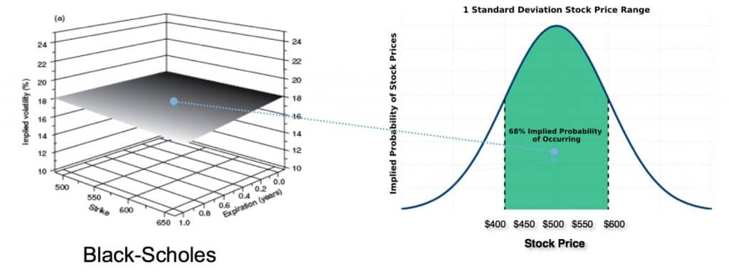
The simplest of the option pricing formulas is the binomial option pricing formula which input variables are easily observed, except for one—the variance of the instantaneous rate of return on the stock. Such a value can be inferred from historical data but also through the Black–Scholes formula. Assuming option prices are such that the Black–Scholes model holds on average, then the market price of the option can be substituted in the model to obtain the instantaneous rate of the variance of the stock.
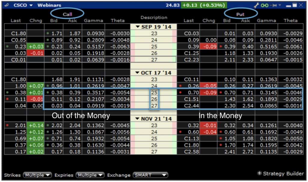
Option’s moneyness. An option is in-the-money if it would be worth something at expiry (provided the underlying’s price did not change), and out-of-the-money in the opposite case. An option at the cross-over point is said to be at-the-money. Moneyness is also employed as a measure (i.e., the log of the distance between the spot and the strike) when considering options on different times to expiration (i.e., normalized on some duration like 3 months, etc.).
The Greeks
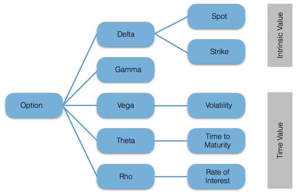
The option’s greeks characterize a contract offering measures of its price sensitivity to the underlying price, the implied volatility, and the option’s strike, time to maturity, and interest rate. However, such measures are forward-looking and represent what can happen to the option’s price whenever such variables change; indeed, greeks do not determine the current price of an option and do not enter the option pricing process. Moreover, the option’s new value is fairly and accurately predicted by the greeks only for small market changes; thus, most hedgers trade the movements of the Greeks rather than the option’s price movements.
Delta is the amount an option price is expected to change based on a 1$ increase in the price of the underlying. The delta is constantly changing because the underlying price is constantly changing. Delta can be considered the speed at which the option’s price changes. Calls have positive delta, ranging between 0 and 1, whereas Puts have negative delta,
ranging between 0 and -1. As a term of comparison, delta for a future contract on the same underlying is approximately 1 because it is expected the future contract to exactly track the underlying. Example: the underlying is trading at 100, the call option at 3.154, delta is 51.6. A drop of 1 in the underlying results in a drop of 0.516 in the option’s value: 99 -> 2.638 and 98 -> 2.122. Note that by definition put option’s delta is negative, thus, for a put option, the example above results in a price increase. Delta can be considered a good approximation for one call option’s probability to expire ITM; thus, delta 51.6 approximate Pc(ITM) at expiration as 51.6%. Instead, one ATM call option has a delta of 0.5 since both alternative states (ITM, OTM) are equally likely, whereas one OTM option has Pc(ITM) < 0.5 and smaller as it is more OTM. Finally, a portfolio of N ATM calls has deltaPc(atm) = N x deltac(atm) = N x 0.5; because for futures deltaF = 1, then the deltaPc(atm) is delta-equivalent to a N/2 portfolio of futures on the same underlying. Thus, by going long on N ATM calls and going short on N/2 futures the resulting delta is 0 and the resulting portfolio is said to be delta-hedge (i.e. no profit or loss is incurred from underlying’s changes).
- Time affects delta proportionally to time’s impact on the probability the underlying’s price can assume values affecting the option’s change in moneyness. For instance, an ITM option, an ATM, and an OTM option with t=1000 have P(XTM)=P(YTM)=0.5 since the remaining alternatives are equally likely. Instead, a deep OTM or ITM option with t=1 has P(ATM)=P(ITM)=0 or P(ATM)=P(OTM)=0 since a sudden and wide change is not probable; however a deep OTM or ITM option with t=1 has P(OTM)=1 or P(ITM)=1 because it is unlikely a sudden and wide price movement. However, an ATM option with t=1 or t=1000 has P(ITM)=P(OTM)=0.5 because both states can still occur with the same probability. Charm is the sensitivity of delta to a change in time.
- Similarly, volatility affects delta proportionally to volatility’s impact on the probability the underlying’s price can assume values affecting the option’s change in moneyness. Vanna is the sensitivity of delta to a change in volatility.
Gamma is a numerical measure of how sensitive the delta is to a change in the underlying. When gamma is large, the delta changes rapidly and cannot provide a good approximation of how much the option moves for each unit of movement in the underlying. Gamma is larger when there is more uncertainty about whether the option will expire in- or out-of-the-money. This means that gamma will tend to be large when the option is at-the-money and close to expiration and smaller for ITM and OTM options; thus, delta will be a poor approximation for the option’s price sensitivity when it is at-the-money and close to the expiration day. Gamma can be considered the responsiveness at which the option’s price changes. Long positions have usually positive gamma, whereas short positions have negative gamma. Example: the underlying is trading at 100, the option at 3.154, delta is 51.6 and gamma is 5. A drop of 1 in the underlying results in a reduction of 5 in the delta: 98 -> 41.6
- Time affects gamma proportionally to time’s impact on the probability the underlying’s price can assume values affecting the option’s change in moneyness. Thus, when time implies a constant probability or delta (0, 0.5, and 1) gamma will be 0; instead, when time implies a change in probability or delta gamma will be positive. Specifically, an ATM option with t=1 incurring in a price movement changing its moneyness implies a change in delta from 0.5 to 1; thus, gamma increases to 0.5. Color is the rate of change of gamma with respect to time.
- Similarly, volatility affects gamma as above. Indeed, a sudden increase in volatility for an ATM option with t=1 implies a wider price movement that may change the option’s moneyness determining a positive gamma.
Rho is the sensitivity of the option price to the risk-free rate, the continuously compounded rate on the risk-free security whose maturity corresponds to the option’s life. The continuously compounded risk-free rate used in the Black-Scholes-Merton is the natural log of 1 plus the discrete risk-free rate. Technically, the Black-Scholes-Merton model assumes a constant risk-free rate; moreover, little change occurs in the option price over a very broad range of the risk-free rate. Theta value is negative when you buy an option and positive when you sell an option. Instruments, such as stocks, whose values are not degraded by time, have zero Theta. The call price increases as the interest rate increases and the put price decreases as the interest rate increases. The reason for this has to do with the cost of carrying the position over time. Just the reverse occurs when interest rates fall. Vera is the rate of change of rho with respect to volatility.
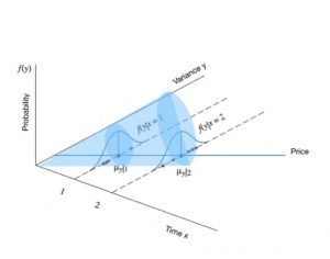
Theta is the rate at which the time value component of the option’s price decays as the option approaches expiration. As represented in the diagram above, time value is a function of the option’s moneyness, its time to expiration, and of the volatility (greater uncertainty corresponds to greater time value). However, since the option price decreases as time moves forward, the theta will be negative and increasing exponentially. Theta is negative for option’s buyers and positive for option’s sellers. Example: The underlying is trading at 100, an option is valued 3.154 with 200 days to go and theta is 42, 51, 64, 1.50. Every 50 days the option’s value decreases to 2.734, 2.644, 2.514, 1.654. Increasing implied volatility makes theta effect more dramatic.
Vega is the amount an option’s price change for a 1% change in implied volatility; it is positive for both calls and puts. Example: The underlying is trading at 100, an option is valued 3.154 with Vega of 43. Thus, a 1% increase in implied volatility results in the option’s values increasing to 3.584. However, vega changes proportionally to the volatility’s impact on the option’s probability of changing its moneyness. Thus, vega is larger the closer the option is to being at-the-money and the longer the option is from expiration. Long positions have always positive vega, whereas short positions have negative vega. The Vega is also a good proxy for the bid-offer spread. The difference between the option’s market price and intrinsic value is given by the Theta premium and Vega premium.
- Time affects vega proportionally to time’s impact on the implied volatility of underlying returns; indeed, the closer at expiration is the option, the lower the relative implied volatility since its lower the option’s probability of changing its moneyness. For instance, annual implied volatility of 18% determines a 1 day implied volatility of 18/(365)0.5 = 0.95%, thus an option with 1 year expiration has vega much larger than the same option with 1 day expiration. Veta is the rate of change in vega with respect to time.
- Volatility affects vega proportionally to volatility’s impact on the option’s probability of changing its moneyness. For an ATM option, the probability does not change, thus vega = 0; however, for ITM and OTM options, vega increases with an increase in volatility since greater implied volatility progressively impact the option’s probability of changing its moneyness. Volga or Vomma is the rate of change in vega with respect to volatility.
Volatility and its Statistical Properties
In general, it does not exist a single definition or concept of volatility concept but rather a family of concepts related to the notion of an undirected dispersion/risk measure.
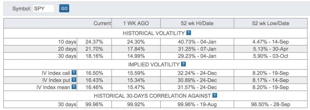
- historical volatility refers to the standard deviation of log-returns of a financial time series. It refers to the past and does not suggest anything about the future; with respect to options, it is computed on the underlying.
- implied volatility is the volatility that, if put into the Black-Scholes-Merton option pricing formula, gives the market-observed price of an option. It is the market’s expectation of future volatility for the underlying; as a result, it often overstates the actual move of the underlying. Usually, it is given as a function of constant maturity (30, 60, 90, and 120 days) and based on ATM calls and puts.
- instantaneous volatility refers to the volatility factor of a diffusion process; for example, in the Black- Scholes-Merton model the instantaneous volatility σ is found in the respective (risk-neutral) stochastic differential equation (SDE). An unadjusted Black-Scholes proxy (or any other model) in which the implied volatility of a short-maturity at-the-money option can be used in place of the true instantaneous volatility state variable. The use of this proxy is justified in theory (Ledoit Lemma) by the fact that the implied volatility of such an option converges to the instantaneous volatility of the logarithmic stock price as the maturity of the option goes to zero. It is seldom seen in common trading settings.
- implied forward volatility between time t1 and t2 is the expected volatility inferred from spot implied volatilities at time (t0 and t1) and (t0 and t2). The procedure is similar to bootstrapping the forward rate from zero-coupon bonds.
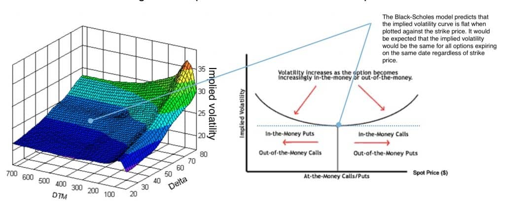
Note that market makers quote (or estimate) for each contract a bid-ask price actually determining two prices or two vols; such spread is where the bank makes its profits and the true price is somewhere in between (and determines another reason to dig deeper into option pricing). If we collect data on implied vols and compare these to historical vols, we note that vols implied by the market prices of options are higher than historical vols and that two different options on the same underlying with the same expiry date can imply different vols. Indeed, if one plots the implied volatility as a function of the strike of an option, one obtains a curve which is roughly smile-shaped. It seems an arbitrage opportunity, but such smiles are a persistent feature of the markets and do not disappear with time. Indeed, the smile expresses the market’s view of the imperfections of the Black-Scholes model.
Specifically, the implied volatility surface for stock indices has the following statistical properties:
- smiles: option implied volatilities exhibit a smile form, i.e. for calls the OTM implied volatilities are higher than the ATM ones; sometimes they rise again for ITM options; this is a phenomenon present in the financial markets mainly since the market crash of 1987. Before the smiles were much shallower but the 1987 crash seems to have triggered a much greater use of options in hedging against jump-risk which increased the smile’s slope because greater demand for out-of-the-money put options from fund managers increases the short-term jump-intensity that in turn increases skewness in the short-dated smiles.
- term structure: smiles are more pronounced for short-term options than for longer-term options; a phenomenon sometimes called volatility term structure
Volatility in-general has the following statistical properties:
- Volatility clusters.
- Volatility mean reverts.
- Stock returns are not normally distributed. In particular, the return distribution has fat tails.
- Volatility tends to increase as the underlying price declines.
- Volatility and volume are highly correlated.
- Volatility is approximately log-normally distributed.
Smiles and Options Models
Smile dynamics are affected by two factors: how the smile changes with spot, and how the smile changes with time. When the implied volatility smile does not change as spot changes is said to be sticky; otherwise the smile floats with spot and the smile is said to be floating. Markets smiles vary as we may expect:
- The equity smile is said to float because its principal cause is the risk-aversion of investors against rapid downward movements; it is highly skewed, much sharper for short maturities and is much flatter for long maturities than for short maturities. These behaviors persist over time. Such features are modeled with a jump-diffusion model.
- The foreign exchange smile is more constant as a function of maturity. It displays a `U’ shape for each maturity but these `U’ shapes are roughly similar for each maturity. The FX smile between major currencies is fairly symmetric and time-constant. Such features are modeled with a stochastic-volatility model with rapid mean-reversion and, as there is no skew, uncorrelated volatility.
- The interest-rate smile has two components: the first is a downward slope which appeared in the mid-1990s; the second component is a slight upward curve for out-of-the-money caplets which appeared in the aftermath of the Asian crisis in 1998. This component reflects risk-aversion to large market moves and is fairly homogeneous across maturities existing even for very long-dated options, for example, ten-year caplets.
In general, many different models are available to fit the empirical shape of smiles, as well as to impose a future change in the smile: a log-normal jump-diffusion model with constant parameters or a stochastic-volatility model with constant parameters have everything defined relative to the current value of spot and time. However, in stochastic-volatility models, it is expected the smile’s shape and level to evolve, even if risk-preferences do not change. A Variance Gamma model with constant parameters, everything is defined relative to the current value of spot and the current time but the smile is symmetric, unlike a jump-diffusion smile. Displaced diffusion models will result in a downward sloping smile. It is a quite sticky smile in that the shape is quite insensitive to the value of spot. The overall level will change a little but if one rescales volatility so that the smile is at the same level then one obtains an almost identical smile. Dupire/Derman-Kani model is fairly constant for large t, that is the model predicts that smiles are destined to disappear. As smiles have persisted for a long period of time, this is an undesirable feature. The other aspect of the model is that the volatility function or is highly dependent on spot. This means that as spot changes, the predicted smile will change greatly, in possibly strange ways. The issues surrounding the pricing of derivatives in a non-Black-Scholes world are still very current and the ideas presented here reflect the debates that are currently going on rather than represent the `correct’ model.
Option’s Pricing Models in Practice
Considering a model for derivatives over an index (statistically less bothering than a single stock), a market model of practical use should at least:
- replicates the most important statistical properties of the index and of the interest rate to be modeled; for instance, implied volatility stochasticity, mean reversion, clustering, leverage effect, volatility smile, volatility term structure, jumps, interest rates positivity, stochasticity, mean reversion, and term structure
- be able to replicate market prices of different instruments, like European options, bonds, or swaps
- have sufficient parameters to calibrate it to market prices or implied volatilities and the yield curve
The general framework of Bakshi, Cao and Chen (1997, BCC97, Bakshi et al. (1997)) explicitly models all major market risks that affect equity derivatives; it can be used in practice for the valuation of any contingent claim and for hedging equity derivatives. Indeed, it can be calibrated to observed market prices by setting its many parameters. BCC97 includes as special cases:
- Black-Scholes-Merton (1973, BSM, Black and Scholes (1973) and Merton (1973)): a model based on geometric Brownian motion with constant volatility and short rate
- Merton (1976, M76, Merton (1976)): extension of BSM with a log-normally distributed jump component
- Heston (1993, H93, Heston (1993)): model including stochastic volatility and constant short rate
- Bates (1996, B96, Bates (1996)): extension of H93 with jump component
Traded securities are a risky stock index S and a risky unit zero-coupon bond B employed to replicate any other security. The risk-neutral dynamics of the stock index S are according to the stochastic volatility jump-diffusion model of Bates (1996, B96). The parameters of the model include:
- the index level at date t
- the risk-less short rate at date t
- the drift correction for jump
- the variance at date t
- the speed of adjustment of the variance to the long-term average of the variance
- the long-term average of the variance
- the volatility coefficient of the index’s variance
- standard Brownian motions
- a Poisson process with a specified intensity
- jump at date t with a cumulative distribution function of a standard normal random variable
- the stochastic short rate of Cox, Ingersoll, and Ross (1985, CIR85, Cox et al. (1985)) with
- a specified speed of adjustment of the rate to the long-term average of the short rate
- the long-term average of the short rate
- the volatility coefficient of the short rate
- a standard Brownian motion
The general market model BCC97 successfully accomplishes the following goals:
- efficient valuation of vanilla options; in general, the preferred choice is the Fourier transform method in combination with numerical integration (FFT)
- calibration of model parameters: equipped with the above, the model can then be calibrated to observed market quotes of such instruments in order to derive a single martingale measure for the valuation of other (exotic) index derivatives
- valuation by simulation: in general, numerical methods are necessary to value the majority of (exotic) equity derivatives; Monte Carlo simulation (MCS) is the most flexible one with the Least-Squares Monte Carlo (LSM) algorithm (cf. Longstaff and Schwartz (2001)) allowing for the incorporation of early exercise features (American style). Moreover, market-based valuation of options and derivatives not liquidly traded can be obtained by calibrating the model to the market quotes of liquidly traded options and then use such a calibrated model for pricing the non-traded options.
- dynamic delta hedging: relying on the LSM algorithm, it is possible to numerically estimate deltas for (exotic) equity derivatives even with American exercise; however, due to market incompleteness (e.g. because of jumps) delta hedging on a stand-alone basis is generally insufficient to hedge or replicate equity derivatives sufficiently well in the general market model of Bakshi-Cao-Chen (1997)
Simplifying, valuation algorithms and models discriminate between the exercise style of the instrument (European or American). Options with European exercise can be priced in three ways:
- PDE method, requiring to solve a partial differential equation (PDE) that a derivative asset must satisfy given the dynamics of the underlying;
- Fourier-based pricing, requiring to derive analytical pricing formulas (integrals) via Fourier transforms
- Monte Carlo simulation, requiring the generation of random process evolutions to derive values for the derivative at maturity; a consistent number of iterations, discounting each simulated option value at maturity, and averaging all discounted option values yields an estimate of the option value
Options with American exercise are generally valued in backward induction (i.e. estimating the option continuation value at maturity and working back to); however, the Least-Square Monte Carlo Simulation employs an OLS regression to estimate the continuation value on the cross-section of the simulated paths. Specifically, the LSM is by construction a lower bound to the mathematically correct America option price; thus, in conjunction with dual methods providing the upper bounds, it offers a range for the true American option value. Thus, a general valuation approach can be substantially translated into the modeling of all risk factors and into the use of a unique numerical method (Monte Carlo Simulation) assuming sufficient computing resources.
References
Hilpisch, I. (2017). Derivatives Analytics with Python
Chance, D. M. (2003). Analysis of Derivatives for the CFA Program
Joshi, M. S. (2015). The Concepts and Practice of Mathematical Finance
Wilmott, P. (2007). Paul Wilmott Introduces Quantitative Finance
Ledoit, 0. (2002). Relative Pricing of Options with Stochastic Volatility