Optimization
Optimization theory has developed from the earliest approaches of De Fermat, Lagrange, Newton, and Gauss through the formalization of Linear programming in 1939 by Kantorovich, the Simplex method of Dantzig and the Duality Theory of von Neumann in 1947, and the Karush-Kuhn-Tucker condition in 1951. Its application disrupted logistics, banking, and economics. In 1960, the introduction of Holland’s Genetic Algorithms and Simulated Annealing in 1983 saw the growth of parallel methods not requiring gradients or higher derivatives. Since the 1990s, AI-based approaches emerged and have matured in recent years.
What is Optimization?
Optimization theory can be defined as science in itself having as field of investigation specific entities named mathematical optimization problems. Such mathematical objects have an unstructured form that often corresponds to a set of functions; specifically, an optimization problem is one where the values of an objective function are to be maximized or minimized over a given set of decision variables and decision functions.
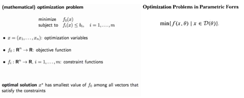
A solution to the problem is the point representing the minimum value assumed by the objective function over all the other possible values constrained by the decision variables. In other terms, the set of decision variables and functions constrain the possible input values for the objective function as well its output values. Specifically, named D the set of points resulting from the application of the constraints, we have through the objective function the image of D and we are searching for a point x i) that belong to D and ii) that corresponds to the minimum in the image of D. Note that a solution might not exist for a specific set D because f(x) does not belong to the image of D, because the minimum in the image of D has not a corresponding point in the domain of the objective function, or because the image of D has not a well defined minimum. Two important theorems ensure that a minimum problem has a dual representation as a maximum problem (and viceversa) and that a transformation that leaves the solution unaffected always exists.
Practical Applications
In practice, optimization theory starts with the identification of the best set of constraints for which the existence of the solution is guaranteed and the characterization of the set of optimal points. Typical problems include:
- Utility maximization in consumer theory (the constraints are income, prices, and budget; the solution is a vector of weights assigned to the set of goods)
- Expenditure minimization
- Profit maximization in producer theory (the constraints are inputs and outputs quantities for a given production function, the market demand function; the solution is a vector of weights assigned to inputs)
- Cost minimization
- Consumption-Leisure choice
- Portfolio choice maximizing utility (the constraints are expected utility and variance; the solution is a vector of weight assigned to the securities uniquely identifying a portfolio)
- Identifying Pareto Optima (i.e., an optimum that satisfies the maximum number of agents)
- Optimal provision of public goods
- Optimal commodity taxation
- Device sizing in electronic circuits (the constraints are area, timing and manufacturing limits; the solution is a vector of weights describing power consumption)
- Data fitting (the constraints are prior information and parameter limits; the solution is a vector of weights describing prediction errors)
- Least squares ( a special case of convex optimization)
Under various theoretical results it is possible to characterize practical problems to ensure that:
- maxima and minima actually exist (Weierstrass Theorem, which provides a general set of conditions)
- Unconstrained optima
- local optima exist (necessary conditions for optima using differentiability assumptions on the underlying problem)
- necessary conditions for local optima expressed as equality constraints (Theorem of Lagrange)
- necessary conditions for local optima expressed as inequality constraints (Theorem of Kuhn and Tucker)
- Convexity conditions for the existence of local optima
- Continuity and monotonicity between the domain and of the objective function and its image
- problems in which the decisions taken in any period affect the decision-making environment in all future periods with a finite horizon (dynamic programming) and infinite horizon (Bellman equation). A notable example in this class is the neoclassical model of economic growth
References
Sundaram, R.K. (1996). A first course in optimization theory