Portfolio analysis statistical considerations
Portfolio analysis is essentially a statistical technique. However, because the ‘‘true’’ population parameters for the input data (expected returns, variances, and covariances) are unobservable, sample statistics must be estimated. Thus, the efficient portfolios generated by portfolio analysis are no better than the statistical input data on which they are based.
Three methods are used for generating the statistical inputs:
- The parameters may be directly estimated on an asset-by-asset basis without assuming any return-generating process
- A one-factor return-generating process can be used to estimate the parameters
- A multiple-factor return-generating process can be assumed to exist, from which the parameters may be estimated
A key assumption of the single-index market model is that the covariance between the error terms of any two securities is zero, thus the covariance of returns between any two securities arises primarily through their relationship with a common market factor. However, if some relevant omitted variables exist, the covariance of returns between any two securities arises through their common relationships with more than a single common factor: for instance the growth rate in the index of the nation’s industrial production. That is, security returns could be assumed to be related to both a market factor and an industrial growth factor:
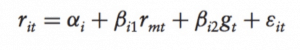
The two-index model can be constructed so that the two independent variables, r and g , are orthogonal by removing the market effect from the growth rate in the index of industrial production. In such case, their covariance is zero. Furthermore, such indexes are assumed to be uncorrelated with the error term. The orthogonalization procedure for removing each factor’s effect on the other factor can be extended to any number of indexes, and essentially consists of the substitution of each index with the residuals of its regression against the other indexes because, by assumption, such residuals are uncorrelated with the other indexes.
As with individual securities, the variance of returns from a portfolio can be decomposed
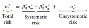
The unsystematic risk will approach zero as the number of individual securities in the portfolio, n, increases. Thus, the total risk of a well-diversified portfolio converges to its systematic risk for large n.
Efficient portfolios can be derived from any return-generating processes by minimizing a Lagrangian objective function:
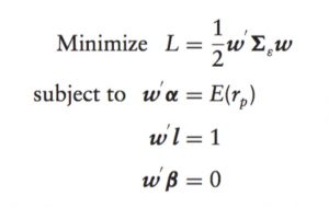
where α’s elements are the intercept terms of the single-index model; β’s elements are beta coefficients for the securities:
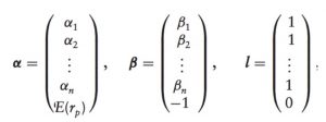
and the matrix:
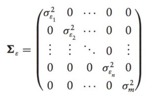
is a variance-covariance matrix of the variances for the error terms and the market. However, the covariance matrix must be a positive definite covariance matrix for the first-order conditions to be necessary and sufficient for a global optimum. Below I briefly explain why:
The non-stationarity of mean and risk
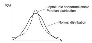
In a dynamic economic environment, firms’ investment and financing decisions will affect the systematic risk, expected return, and standard deviation of returns. For example, Boness, Chen, and Jatusipitak (1974) find parameters shift after a capital structure change and Christie (1982) demonstrates that the standard deviation of a stock’s return is an increasing function of both financial and operating leverage. Beaver’s (1968) realized returns and Patell and Wolfson’s (1981) ex-ante assessments support an increase in the variance of stock returns around the announcement of quarterly earnings. Macro information shocks may also shift the level of interest rates and market risk premiums. Therefore, it is not surprising for the expected return and the risk dimensions of individual stocks and portfolios to change through time. Nonstationarity of mean and risk could cause the skewness, highly peaked, and longer-tailed (leptokurtic) characteristics in the empirical unconditional distribution of asset returns.
Several statistical distribution models can capture the skewness and leptokurtic features of asset returns:
- Stable Paretian distributions are completely characterized by four parameters. The normal distribution is one particular member of what is known as the family of stable Paretian distributions. All members of this family are invariant under addition, meaning that when random variables from a particular distribution are added together, the resulting random variable will have the same distribution. However, if daily returns come from a non-normal stable Paretian distribution (meaning α ̸= 2), then the central limit theorem cannot be invoked and the conclusion that monthly returns will be normally distributed cannot be drawn. Indeed, it has been argued conceptually that the monthly distribution for common stock returns is leptokurtic, meaning the distribution has more observations in the tails and center and fewer in the shoulders relative to the normal distribution. Fama (1965), in a detailed empirical study of daily returns, found that observed returns were leptokurtic and concluded that a non-normal stable Paretian distribution fit the data better than a normal distribution.
- The Student’s t density function of asset returns. Blattberg and Gonedes (1974) argued that the observed leptokurtic daily return distribution can be explained by an alternative to the non-normal stable Paretian distribution, the Student’s-t distribution. Although able to explain the leptokurtosis observed by Fama (1965) in daily returns, the Student’s-t distribution has a finite standard deviation. Thus, the central limit theorem can be applied to it and used to provide an argument that monthly returns are approximately normal. Furthermore, Blattberg and Gonedes, and later Fama (1976), argue that the empirical evidence on monthly returns suggests that normality is a reasonable approximation.
- Discrete Mixtures of Normal Distributions. Because there are good reasons to expect this distribution to be shifting or nonstationary, Kon investigated whether or not daily returns could be modeled as a discrete mixture of different normal distributions in which each return observation is viewed as a drawing from one of a finite number of normal distributions with some probability. He found the mixed distribution model to have more descriptive validity than the Student’s-t distribution. For instance, the cycle time required for traders to define a strategy, enter the market, assess, and exit is generally not normally distributed, nor does it have a lognormal distribution. Thus, the complex trades represent all the longer times, while the simpler contracts have shorter times.
- Sequential Mixtures of Normal Distributions. Relevant information that changes the risk-return structure is randomly released within some time interval in sequence. These information events translate into sequential discrete structural shifts for the mean and/or variance parameters in the time-series of security returns. Research showed the sequential mixture specification has substantially more descriptive ability than the competing alternatives (normal distribution, Student’s-t distribution, discrete mixture of normal distributions, and Poisson jump-diffusion process model).
- The Poisson jump-diffusion process for the distribution of stock returns consists of a geometric Brownian motion component and an independent compound Poisson process with normally distributed jump amplitudes.
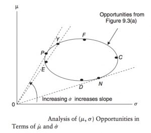
- Lognormal distribution. One argument against normality is based on the concept of the investor’s limited liability: investors cannot lose more than the value of their investment. This suggests that returns are likely to be generated by a positively skewed distribution. If the assumption of normality is replaced by an assumption of lognormality and investors are assumed to have utility functions displaying positive marginal utility of wealth then the efficient frontier theorem is still useful. The efficient portfolio f in the Risk-return Space (μ ̇ , σ ̇ ) for continuously compounded returns is the portfolio with the maximum expected return in the long run. That is, efficient portfolio f has the maximum geometric mean rate of return because E(ln(1 + r)) = μ ̇ is a geometric mean return. It also corresponds to the optimal portfolio for an investor with a logarithmic utility function and will lie between E and F (the traditional efficient frontier) in the opportunity sets in Risk-return Space (μ, σ ) for non-compounded returns. The portion of the (μ, σ) efficient frontier along the curve EP in the figure above is not (μ ̇,σ ̇) efficient. That is, a part of the traditional efficient frontier is no longer efficient if returns are lognormal. If a risk-free borrowing and lending rate exists, then there is no difference in the efficient frontiers because the tangency points are identical. As a result, under these circumstances, the CAPM still holds if returns are lognormally distributed. In conclusion, the (μ, σ )-efficient frontier contains some undesirable portfolios in its highest and lowest return sectors that are eliminated in the logarithmic transformation to the (μ ̇,σ ̇)-efficient frontier. The (μ ̇ , σ ̇ ) analysis, however, includes and eliminates the positive skewness of the discrete holding period returns in deriving the continuous- time efficient frontier and is thus a superior decision-making process. Finally, the (μ ̇,σ ̇) analysis pinpoints the long-run wealth-maximizing portfolio not present in the (μ, σ ) analysis.
In such circumstances when the mean and variance parameters are not sufficient to describe the investment environment, other portfolio selection criteria are used: the geometric mean return (GMR) criterion, the safety-first criterion, value at risk (VaR), copulas, semivariance, stochastic dominance, and the mean-variance-skewness criterion.
Returns Distribution Fitting
Substantially, estimating the best stable Paretian distribution is rather daunting. A common method fits a number of distributions to sample data, compare the goodness of fit with a chi-squared value, and test for significant difference between observed and fitted distribution with a Kolmogorov-Smirnov test. The chi-squared value bins data into 50 bins based on percentiles so that each bin contains approximately an equal number of values. For each fitted distribution, the expected count of values in each bin is predicted from the distribution. The chi-squared value is the sum of the relative squared error for each bin, such that:
chi-squared = sum ((observed – predicted)2) / predicted)
The cumulative sum of observed and predicted frequency across the bin range used are employed for the observed and predicted parameters above. The lower the chi-squared value the better the fit. The Kolmogorov-Smirnov test assumes that data has been standardized (demeaned and then divided by the standard deviation). A value greater than 0.05 means that the fitted distribution is not significantly different from the observed distribution of the data.
However, when working with large datasets of real-world data often no theoretical distribution fits the data perfectly or, even worst, the theoretical distribution does not match the process generating the data; indeed, statistical distributions are theoretical models of real-world data that closely match the underlying generating process. In practice, the theoretical model and the test must both agree.
Accordingly to the code above, the Weibull distribution formula is selected to model the log-returns of the S&P500 over the last 18 years. The theoretical model is used to measure the mean-time of failure of a piece of equipment in the production process. Thus, we can accept the model to predict how many failures will occur in the next quarter, six months, or year for the purpose of forecasting tail risk measures as VaR.
References
E. Elton, M. Gruber, S. Brown, W. Goetzmann. (2007). Modern Portfolio Theory and Investment Analysis, 11th edition.