Capital Allocation Methods

Capital allocation methods are used to estimate risk margins in the form of return on equity (ROE) measurements and targets from a top-down perspective. Actuarial risk theory views risk from a bottom-up perspective because it aims at modeling solvency. At a macro level, financial theory views capital as the equity capital supplied by investors.

Kulik

Capital allocation evolved in such context with a final reconciliation and theoretical equivalence of capital allocation and risk load methodologies. Solid asset allocation is the objective of any methodology; however, the effectiveness of a capital allocation methodology can only be evaluated within its intended perspective. Consider the followings:

• a traditional allocation is 60% World Stock Market Index (Vanguard Total World Stock Index Fund NYSE: VT) and 40% Bond Market Index (Vanguard Total Bond Market Index Fund NYSE: BND)
• an equal weight portfolio 34% Stock Market Index (Vanguard Total Stock Market Index Fund NYSE: VTI) 33% Bond Market Index (Vanguard Total Bond Market Index Fund NYSE: BND) 33% International Stock Market Index (Vanguard Total International Stock Index Fund NYSE: VXUS)
• a conservative portfolio 25% Large Cap Stocks (Vanguard Large Cap Index Fund NYSE: VV) 20% Small Cap Stocks (Vanguard Small-Cap Index Fund NYSE: VB) 5% International Stock Market Index (Vanguard Total International Stock Index Fund NYSE: VXUS) 40% Intermediate-Term Bonds (Vanguard Intermediate-Term Bond Fund NYSE: BIV) 10% Short Term Bonds (Vanguard Short Term Bond Fund NYSE: BSV)
• an aggressive portfolio 30% Large Cap Stocks (Vanguard Large Cap Index Fund NYSE: VV) 30% Small Cap Stocks (Vanguard Small-Cap Index Fund NYSE: VB) 20% International Stock Market Index (Vanguard Total International Stock Index Fund NYSE: VXUS) 10% Emerging Market Stocks (Vanguard Emerging Markets Index Fund NYSE: VWO) 10% Bond Market Index (Vanguard Total Bond Market Index Fund NYSE: BND).

The two main components of investment strategy are Strategic Asset Allocation (SAA) and Tactical Asset Allocation (TAA). SAA sets the long-term asset allocation for the portfolio while TAA adjusts the asset allocation to short-term considerations, such as risks and investment opportunities. Investment strategy also covers investment selection, to populate each asset class with appropriate investments, and risk management.

For example, the long-term investment objectives may be beating inflation and growing the portfolio by 2% per annum. The investment constraints are excluding bonds below investment grade and alternative investments. The investment strategy may thus include SAA that allocates the portfolio to asset classes that keep up with inflation (e.g. inflation-linked bonds) and asset classes that provide growth over the long term (e.g. equities). Commodities, whose value normally increases with inflation, are excluded due to the constraints that do not permit investing in alternative investments. The expected return of the asset allocation is 4.5% per annum (2.5% for inflation and 2% for real return). TAA tweaks the allocation between equities and bonds based on the stage in the economic cycle and the view on whether equities should outperform or underperform bonds over the short term. Investment selection picks the actual investments under each asset class (e.g. active or passive equities) and ensures that all bonds are above investment grade, as per the constraints. Risk management guides the portfolio to the investor’s risk tolerance. The required risk level is not too high (the return objectives are relatively conservative), while enough risk should be taken to achieve the objectives.

Capital allocation methods

Traditionally, Markovitz’s Modern Portfolio Theory established a formal risk/return framework for investment decision-making, asset selection, and portfolio management by defining investment risk in quantitative terms. However, the framework has been continuously criticized since its introduction; substantially, PMPT and research in Behavioral Finance (CPT) had pointed the way showing how to apply the PMPT to improve investment results and to upgrade the MPT principles to a new level of usefulness.

• According to MPT, securities should be analyzed in terms of how they interact (correlate) with other elements of a portfolio in order to construct a portfolio with the same expected return but lower risk. MPT models risk using standard deviation above and below expected returns. Client objectives are translated into a return figure that brings current assets plus future cash flows to a desired terminal wealth. Then, with this return, MPT suggests the lowest risk asset mix. In practice, assets’ percentage allocations are largely a function of the investor’s risk tolerance; MPT is essentially a buy-and-hold strategy (apart from rebalancing). Its performance measure is the Sharpe ratio.
• PMPT models risk using only standard deviation below expected returns (semivariance). In other words, MPT assumes that there is such a thing as upside risk, whereas PMPT proponents believe that only downside risk matters to investors. The focal point is not the maximum return possible given a certain level of risk, but rather the rate of return that must be earned in order to accomplish the customer’s specific investment goals with minimum risk. As a result, returns below the target rate of return (“downside risk”) incur risk; returns above the target do not. Its performance measure is the Sortino ratio.
• Research in Behavioral science promoted CPT in order to account for investors greater hate for loss than enjoyment for gain; such asymmetry induces the management of downside risk by overlaying portfolio insurance on an asset mix (derivatives, market timing with tactical or rotational asset allocation, etc.).

The central idea of the Risk Parity approach is that in a well-diversified portfolio all asset classes should have the same marginal contribution to the total risk of the portfolio. In this sense, a risk parity portfolio is an equally weighted portfolio. Additionally, the approach relies on accurate estimates of volatility which have been to shown to be relatively stable.

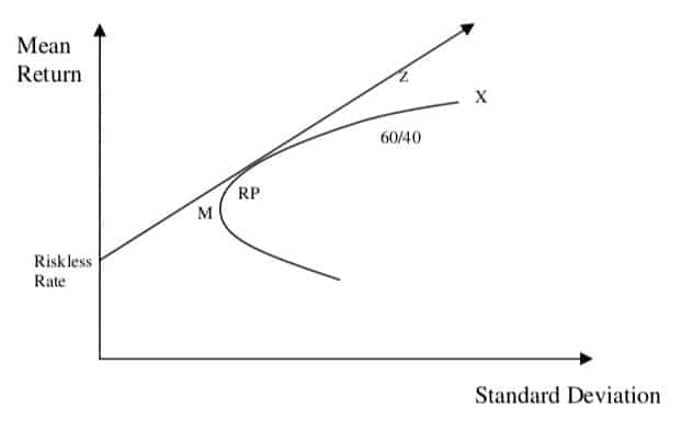
A risk-parity portfolio RP would have performed very well during the last 20 years with an annualized rate of return of 7.12%. This is roughly equal to the annualized rate of return on the 60/40 portfolio with a volatility that is 50% smaller than that of the 60/40 portfolio.

• However, portfolio Z, which is a combination of the risk parity portfolio RP and leverage, has the same risk as the 60/40 portfolio but with a higher expected rate of return. However, if the risk parity portfolio is far away from the efficient frontier, the leveraged approach to risk parity asset allocation may lead to poor performance. In other words, it is critical for the risk parity portfolio to be close to the efficient frontier.

• The key is for the low volatility portfolio to have a Sharpe ratio that is higher than the 60/40 or other high volatility portfolios. If the Sharpe ratio of the low volatility portfolio is lower than the riskier portfolio, then leverage will actually lead to a portfolio that will be inferior to the riskier portfolio.

A Volatility-Weighted approach considers the weight of each asset class proportional to the inverse of its volatility. This approach is identical to the risk parity approach when we have only two assets and it will be the same as risk parity in the more general case if correlations between asset returns are the same. Both the volatility-weighted and the risk parity portfolios have much higher Sharpe ratios than the 10/50/40 portfolio; thus, if levered up to have the same volatility as the 10/50/40 portfolio, they will have higher mean return than the 10/50/40 portfolio.

• the allocations to alternative investments will be relatively high in a risk parity portfolio because they have low volatility and low correlations with other asset classes.
• the volatility-weighted and the risk parity portfolios require significant allocations to hedge funds and bonds
• only investors who are able and willing to use derivatives may lever up their risk parity portfolios

Risk parity and volatility weighted effectively bridge the gap between two foundational concepts in modern finance: the belief in efficient markets, and Modern Portfolio Theory (MPT). That’s because a Risk Parity portfolio delivers the most efficient returns when investors have priced markets appropriately, such that major asset classes are expected to deliver returns in proportion to the amount of risk each contributes to the portfolio. Investors who do not fully understand risk parity strategies often are concerned that the strategy’s higher exposures to fixed income will cause it to underperform traditional portfolios with more equity exposures over the long run. This is only true in situations where investors cannot use leverage.

The Kelly’s Criterion is well known among gamblers and investors as a method for maximizing the returns one would expect to observe over long periods of betting or investing. Kelly’s Criterion can be used to calculate
optimal returns and can generate portfolios that are similar to results from the Mean Variance-model; moreover, it can be used in either discrete finance or continuous finance applications. Substantially, Kelly’s Criterion is used to guide an investor to take more risk when investments are winning and cut risk when investments’ returns are deteriorating; thus, Kelly’s Formula is used to calculate optimal capital allocation between different investments and the optimal leverage of a portfolio.

• The objective of the related optimization problem is to maximize long-term wealth which is equivalent of maximizing the long-term compounded growth rate g of the portfolio. The objective means that ruin (equity going to zero) must be avoided.
• The main advantage of the Kelly criterion, which maximizes the expected value of the logarithm of wealth period by period, is that it maximizes the limiting exponential growth rate of wealth. The main disadvantage of the Kelly criterion is that its suggested bets may be very large. Hence, the Kelly criterion can be very risky in the short term. As a result, because of uncertainties in parameter estimations, and because return distributions are not Gaussian, traders prefer to cut recommended leverage to half-kelly for safety.

For long term compounders, the good properties dominate the bad properties of the Kelly criterion. But the bad properties may dampen the enthusiasm of naive prospective users of the Kelly criterion. The Kelly and fractional Kelly strategies are very useful if applied carefully with good data input and proper financial engineering risk control.

The Black-Litterman Model

In a search for a reasonable starting point for expected returns, Black and Litterman (1992), He and Litterman (1999), and Litterman (2003) explore several alternative forecasts concluding that most lead to extreme portfolios. Thus, their model uses “equilibrium” returns as a neutral starting point.

• Consider an index like the UBS Global Securities Markets Index (GSMI), a global index based on capitalization and a good proxy for the world market portfolio; the weights of its constituent are the market capitalization weights
• Equilibrium returns are derived using a reverse optimization method in which the vector of implied excess equilibrium returns is extracted from the formula Π = λ Σ w_mkt where Π is the Implied Excess Equilibrium Return Vector (N x 1 column vector); λ is the risk aversion coefficient; Σ is the covariance matrix of excess returns (N x N matrix); and, w_mkt is the market capitalization weight (N x 1 column vector) of the assets.
• The covariance matrix can be a simple covariance matrix of historical returns. However, investors should use the best possible estimate of the covariance matrix of excess returns. Qian and Gorman (2001) extends the Black-Litterman model, enabling investors to express views on volatilities and correlations in order to derive a conditional estimate of the covariance matrix of returns. They assert that the conditional covariance matrix stabilizes the results of mean-variance optimization.

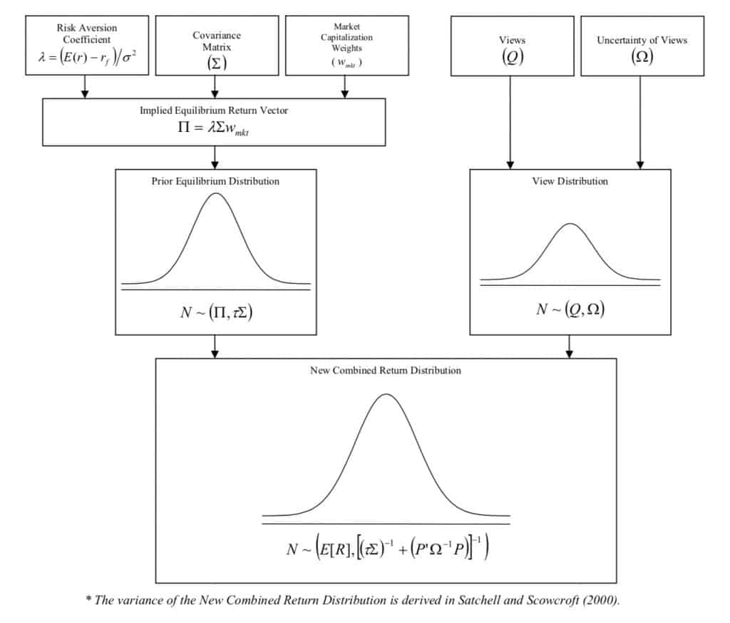
• More excess return per unit of risk (a larger lambda) increases the estimated excess returns. The implied risk aversion coefficient ( λ ) for a portfolio can be estimated by dividing the expected excess return by the variance of the portfolio (Grinold and Kahn (1999)): λ =E(r)−r_f / σ² where E(r) is the expected market (or benchmark) total return; r_f is the risk-free rate;and, σ² is the variance of the market (or benchmark) excess returns.
• The reverse-optimized Implied Equilibrium Return Vector (Π) is based on CAPM returns derived from implied betas (not regression betas). The implied betas are the betas of the N assets relative to the market capitalization-weighted portfolio.

The Black-Litterman model uses a Bayesian approach to combine the subjective views of an investor regarding the expected returns of one or more assets with the market equilibrium vector of expected returns (the prior distribution) to form a new, mixed estimate of expected returns. The resulting new vector of returns (the posterior distribution), leads to intuitive portfolios with sensible portfolio weights. The model overcomes the problem of unintuitive, highly-concentrated portfolios, input-sensitivity, and estimation error maximization.

Conceptually, the Black-Litterman model is a complex, weighted average of the Implied Equilibrium Return Vector ( Π ) and the View Vector ( Q ), in which the relative weightings are a function of the scalar (τ ) and the uncertainty of the views ( Ω ). From a macro perspective, the new portfolio can be viewed as the sum of two portfolios, where Portfolio 1 is the original market capitalization-weighted portfolio, and Portfolio 2 is a series of long and short positions based on the views. Below are three sample views expressed using the format of Black and Litterman (1990):

• Simple views: International Developed Equity will have an absolute excess return of 5.25% (Confidence of View = 25%).
• Relative views: International Bonds will outperform US Bonds by 25 basis points (Confidence of View = 50%). Each row in P must sum to 1 with positive (+1) outperforming and negative (-1) outperforming.
• Portfolio views: US Large Growth and US Small Growth will outperform US Large Value and US Small Value by 2% (Confidence of View = 65%). Outperforming and underperforming will form a small portfolio view with weight proportional to their market capitalization (w_USLG=mc_USLG/(mc_USLG+mc_USLV)); then, the weight is used in P as in relative views.

The uncertainty of the views results in a random, unknown, independent, normally-distributed Error Term Vector (ε ) with a mean of 0 and covariance matrix Ω. Thus, a view has the form Q+ε . The variance of each error term (ω ), which is the absolute difference from the error term’s (ε ) expected value of 0, form Ω, the diagonal covariance matrix.

In order to assess how the confidence level of the views impacts the portfolio, it is possible to compare the vector of the weights of the market with the vector of the weights obtained assigning 100% to confidence levels. Between the two will be the vector of the weights derived with the given confidence levels.

References

E. Elton, M. Gruber, S. Brown, W. Goetzmann. (2007). Modern Portfolio Theory and Investment Analysis, 11th edition.

T. Idzorek (2005). A STEP-BY-STEP GUIDE TO THE BLACK-LITTERMAN MODEL Incorporating user-specified confidence levels.

H. Kazemi. An introduction to Risk Parity

Z. Peterson. Kelly’s Criterion in Portfolio Optimization: A Decoupled Problem

L. C. Mac Lean, E. O. Thorp, W. T. Ziemba (2010). Good and bad properties of the Kelly criterion

Quantra (2019). Quantitative Portfolio Management