Entropy, Incomplete Information, and Machine Learning: What Margins Cannot Tell Us
A company often has reliable totals without knowing how those totals combine. A distributor may know how many units were sold in each region and how many of each product were sold overall, while lacking the product-by-region breakdown needed for replenishment. The question is not simply how to fill a table. It is which conclusions are supported by the available information.
Entropy provides a precise way to describe uncertainty. Maximum entropy is one principled method for selecting a distribution under explicit constraints. It does not, by itself, demonstrate that the resulting distribution represents an unobserved population. This distinction also matters in supervised machine learning, where a model can fit observed data and still fail on new conditions.
The missing information: an inventory example
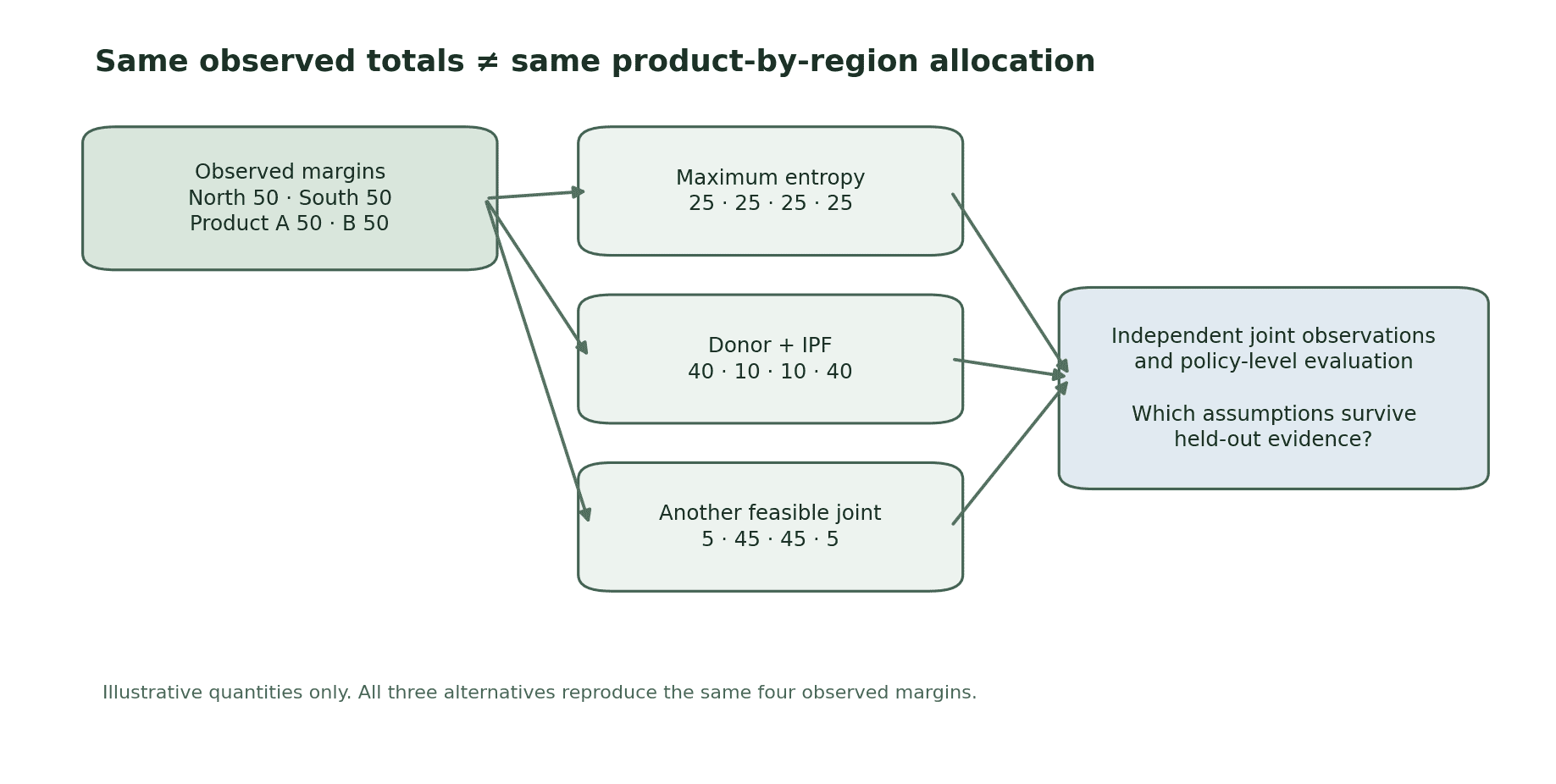
Suppose a company sells 100 units across two regions and two products. Its accounting data provide the following constraints: Region North sold 50 units; Region South sold 50; Product A sold 50; Product B sold 50. The intersection of product and region is unavailable.
A table that satisfies all four totals is:
| Distribution | North: A | North: B | South: A | South: B |
|---|---|---|---|---|
| Maximum-entropy allocation | 25 | 25 | 25 | 25 |
| Donor-pattern allocation | 40 | 10 | 10 | 40 |
| Another feasible allocation | 5 | 45 | 45 | 5 |
All three allocations satisfy the same published totals. Yet they imply very different inventories for the two regions. A national forecast might look identical under all three, while a local replenishment decision could differ sharply. Matching known totals is not the same as identifying the missing joint distribution. The figures above are hypothetical, not measured observations.
Shannon entropy and the maximum-entropy choice
For a discrete probability distribution p, Shannon entropy is:
H(p) = −Σi pi log pi.
Here, pi is the probability of outcome i; the logarithm’s base sets the unit. Entropy is larger when probability is distributed more evenly among the possible outcomes, given the stated support.
The maximum-entropy principle selects the feasible distribution with the greatest entropy, conditional on the constraints and the chosen set of possible outcomes. In this example, with only the row and column totals and a uniform reference measure, the four equal entries maximize entropy. The rule is transparent: it does not add an association between region and product that the data do not require.
But that transparency is not a discovery of independence. If customers in the North actually prefer A, the equal allocation will miss that preference. The constraints alone cannot settle the issue. Shannon introduced the information measure; Jaynes subsequently developed maximum entropy as a principle of inference from partial information.
Donors and iterative proportional fitting: preserve a different assumption
An alternative begins with an empirical donor: a previous detailed sales table, a comparable market, or another population providing a product-by-region pattern. Iterative proportional fitting (IPF, also called raking) repeatedly adjusts the donor’s cells to match the new known margins.
The divergence from the donor describes departure from the reference distribution; it is not a direct measure of error against an unknown real population. If the donor already has entries 40, 10, 10, and 40 and matches the target margins, IPF need not change those entries. The donor-based table and maximum-entropy table then remain different despite exactly matching the same margins.
IPF is therefore not simply a competing algorithm for discovering the same hidden truth. It answers a different conditional question: what allocation satisfies the margins while preserving the donor structure as closely as the method permits? A donor with structural zero cells also restricts what standard multiplicative updates can recover; additional modeling assumptions may be needed to assign probability to those cells.
Where machine learning and cross-entropy enter
Supervised machine learning uses observed input–outcome pairs to estimate conditional relationships. For example, product-level demand observations, promotions, regional characteristics, and past inventory availability could support a model of regional product demand. A learned distribution is useful only to the extent that informative examples and features exist; machine learning cannot identify a missing association from the same marginals alone.
For classification, a common training loss is cross-entropy. This loss penalizes putting little probability on outcomes that occur. Its role differs from maximizing entropy subject to constraints: one fits predictions to labeled observations; the other selects among distributions consistent with partial information. Kullback–Leibler divergence connects the quantities mathematically, but the information inputs and inference targets remain distinct.
A model can have low training cross-entropy and still be poorly calibrated on later demand, a new region, or unusual lead-time conditions. Proper out-of-sample scoring, calibration plots, and relevant decision metrics are needed to assess that risk.
What could actually distinguish the alternatives?
The comparison needs independent information not already used to construct the candidate tables. For a distributor, this might be an audited sample of product-by-region sales, a temporally held-out detailed transaction period, or a controlled additional data collection. For synthetic populations, it could be independent joint counts or held-out cross-tabulations. Without such evidence, one can compare properties and assumptions but not establish which estimated joint distribution is more accurate.
An informative evaluation should report at least four things:
- Constraint fidelity: Do all reconstructed tables reproduce the stated regional and product margins?
- Information provenance: Which additional associations came from a donor, labeled data, or explicit structural assumptions?
- Independent accuracy: On joint cells not used for fitting, how do estimated allocations differ from observations? Consider absolute errors, distributional distances, and uncertainty.
- Decision sensitivity: Would using each allocation lead to different replenishment quantities, transfer plans, stockouts, or distribution costs under the same policy simulator?
An additional intervention—for example, a localized promotion—may reveal relations that marginal totals obscure, but it must be designed and interpreted with the relevant causal assumptions. Merely optimizing the reconstruction objective does not substitute for this test.
Why this matters beyond inventory
The same difficulty appears when reconstructing synthetic households from census margins, estimating demand across demographic groups, allocating resources among service locations, or modeling social and institutional systems under partial observation. A mathematically well-defined estimate is valuable because its assumptions are explicit. It is not equivalent to a verified description of the underlying system.
For an operational team, entropy is best understood as part of a broader information sufficiency audit: identify the decision, list which joint relationships it requires, establish what is observed, compare defensible reconstruction methods, and seek independent evidence for the relationships most consequential to that decision.
Assess What Your Data Can Support
Are you constructing synthetic populations, estimating unobserved relationships, or developing decision models from incomplete datasets?
Bamboos Consulting can help examine information sufficiency, compare statistical reconstruction methods, and evaluate how modeling assumptions influence estimates and simulation outcomes.
The assessment can distinguish what follows from the available data, what depends on methodological assumptions, and what requires independent validation before supporting a decision.
Explore related methods in Machine Learning & Optimization, review our Technical Resources, and find additional analysis on Substack.
References
- Shannon, C. E. (1948). A Mathematical Theory of Communication. Bell System Technical Journal, 27(3), 379–423.
- Jaynes, E. T. (1957). Information Theory and Statistical Mechanics. Physical Review, 106, 620–630.
- Deming, W. E., & Stephan, F. F. (1940). On a Least Squares Adjustment of a Sampled Frequency Table When the Expected Marginal Totals are Known. Annals of Mathematical Statistics, 11(4), 427–444.
- Kullback, S., & Leibler, R. A. (1951). On Information and Sufficiency. Annals of Mathematical Statistics, 22(1), 79–86.
- Gneiting, T., & Raftery, A. E. (2007). Strictly Proper Scoring Rules, Prediction, and Estimation. Journal of the American Statistical Association, 102(477), 359–378.