

Technical Resources / Industrial Computer Vision
A model that identifies visible defects in a benchmark is not necessarily suitable for a specific production line. The practical question is whether it misses unacceptable defects, generates a manageable volume of false alarms, and behaves consistently across batches and acquisition conditions. This article sets out a bounded evaluation protocol for those questions. It describes a test design, not a validated inspection deployment.
1. Start with the consequences of each decision
Suppose one camera images each manufactured item. The model proposes whether a defect is present and a downstream rule may flag the item, clear it, or send it to a human reviewer. A missed defect may proceed to later processing; a false alarm may consume review capacity and delay production. These consequences are not symmetric, and a single accuracy score cannot capture them.
A feasibility study begins by documenting the defect taxonomy, which defects matter most, how labels are adjudicated, the expected operating prevalence, and the available review capacity. The threshold that converts model scores to actions should be recorded before final testing rather than tuned repeatedly on the held-out sample.

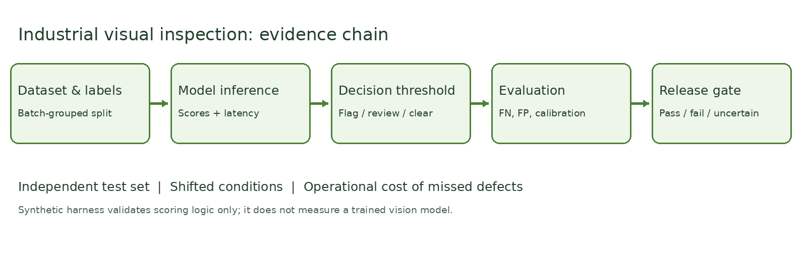
2. Design a dataset that tests generalization
Defect images from the same physical item or production batch can be unusually similar. If such images appear on both sides of a random train/test split, apparent performance may exaggerate generalization. Retain acquisition timestamps, equipment identifiers, production-batch records, lighting settings, and annotation decisions. Where relevant, reserve complete items, batches, acquisition sessions, or cameras for independent assessment.
Defect labels may be uncertain. Borderline or disputed examples should be retained as such, with a documented adjudication rule. Subclasses with severe consequences deserve separate reporting even if rare. Public datasets are useful for methodological comparisons, but their labels and image distributions are not interchangeable with factory-specific operating conditions.
3. Measure defect recall, false alarms, and their uncertainty
Defect recall is the fraction of truly defective items detected. The false-negative rate is the share of defects missed. The false-positive rate is the share of acceptable items flagged as defective. Precision additionally depends on the prevalence of defects in the tested population, so values from artificially balanced datasets may not transfer to actual production.
Report the confusion matrix, denominators by defect subtype, decision threshold, and a confidence interval justified by the sampling process. A run with zero missed defects does not imply a zero probability of future misses: even under independent and identical trials, a finite sample only provides a bound. Adjacent video frames or images from one batch should not be counted as independent items merely to increase the apparent sample size.
4. Challenge the complete inspection path
Tests should include nominal lighting, illumination shifts, blur, occlusions, new batches, changes in camera configuration, and malformed or missing inputs. Beyond image classification, monitor dropped frames, processing delays, queue growth, operator-review volume, missing traces, and recovery after a timeout. A timeout or unreadable image must have an explicit operational outcome; silently classifying it as acceptable would undermine the evidence chain.
Each condition needs a declared number of test items, model and preprocessing version, acquisition configuration, and expected behavior. An accelerated inference comparison using Intel OpenVINO requires real model execution on documented hardware. A synthetic timing variable is not a hardware benchmark.
5. What the accompanying software actually demonstrates
The technical package contains a reproducible Python scorer and 48 synthetic records. The scorer computes confusion-matrix counts and class-sensitive error rates and records nominal versus shifted-condition breakdowns. Eight automated unit tests pass. These observations validate a small scoring implementation, not an image classifier. No real photographs, trained model, camera, or production equipment were used.
For the same reason, the release gate remains inconclusive for real-model performance. Before operational claims can be made, the protocol requires an appropriately licensed dataset, a fixed trained baseline, independently held-out evaluation conditions, actual inference and timing measurements, and a documented risk-based decision.
6. Academic and industrial context
Bergmann et al. (2019) introduce MVTec AD as an anomaly-detection benchmark. Heckler-Kram et al. (2026) describe MVTec AD 2 and more challenging evaluation settings. The MVTec AD 2 dataset has a non-commercial data license; public availability does not authorize its commercial reuse without appropriate rights.
The NIST AI Risk Management Framework supplies general measurement and governance concepts. McKinsey’s 2025 State of AI survey and Deloitte’s 2026 Manufacturing Industry Outlook provide organizational and investment context, not experimental confirmation of this protocol or an inspection model.
Companion technical note: Industrial Computer Vision: Evaluation Protocol (PDF).
For a bounded computer-vision feasibility study, visit AI Consulting & Computational Systems. The broader methods library appears under Technical Resources.