The single index factor model

The single-index factor model assumes that the co-movement between stocks is due to a single common influence or index. Casual observation of stock prices reveals that when the market goes up (as measured by any of the widely available stock market indexes), most stocks tend to increase in price, and when the market goes down, most stocks tend to decrease in price.

The models developed for forecasting correlation structures fall into two categories: index models and averaging techniques. An index model is a Statistical model of security returns (as opposed to an economic, equilibrium-based model). The most widely used technique is the single-index model, an empirical description of stock returns that can represent a linear relationship with any economic variable relevant to the security; however, it assumes only one factor as the cause of the systematic risk affecting returns. The model represents the return of stock i as:

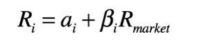
where a, beta, and the market return are random variables. Since alpha represents the component of return insensitive to (independent of) the return on the market it can be expressed by the sum of alpha and a random error quantity e. Thus, the return of stock i is rewritten as:

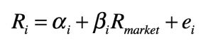
The single-index model assumes that the error e is independent across stocks. Thus, the only reason stocks vary together, systematically, is because of a common co-movement with the market. There are no effects beyond the market (e.g., industry effects) that account for co-movement among securities. Additionally, the single-index model considers that e and the market return R are uncorrelated to specify that the equation describes the return on any security independently from how the return on the market changes. Estimates of alpha, beta, and covariance of errors are often obtained from time series–regression analysis.

The Single Index Model specifies two sources of uncertainty for a security’s return:

• Systematic (macroeconomic) uncertainty (which is assumed to be well represented by a single index of stock returns)

• Unique (microeconomic) uncertainty (which is represented by a security-specific random component)

As a result, empirical implementations require to select an index so that e are uncorrelated for any two assets. A common choice is the S&P500 as the index because the entire stock market (a value-weighted portfolio) is a good proxy to capture all macroeconomic fluctuations.

Finally, the single index model is employed to represent the joint movement of securities in portfolio analysis because it allows to drastically reduce the inputs to the Markowitz portfolio selection procedure (from 2n + (n*n – n)/2 to 3n+2). However:

• The total portfolio variance represents the variance of portfolio returns around the expected return as computed with the single index model.
• The volatility of the portfolio return can be decomposed into three sources: 
  • the sensitivity to the market factor beta
  • the volatility of the market factor
  • the specific risk. 

One of the limitations of the equity beta as a risk measure is that it ignores the other two sources of risk: it says nothing about the risk of the market factor itself or about the specific risk of the portfolio. The canonical risk decomposition rests on an assumption that the benchmark or index is uncorrelated with the specific returns on a portfolio.

How to use the single index factor model

As stated above, alpha, beta, e, and the market return are random variables assumed to be normally distributed. Because of the properties of the normal distribution, the return of the stock is also normally distributed; indeed, returns can be positive or negatives.

However, the prices underlying the returns are not normally distributed; indeed, stocks are assumed to grow at a compounded rate. The valuation of the growth of a company is not relevant here; however, to calculate possible expected prices, an analyst will take the current stock price and multiply it by various normally distributed rates of return (which are mathematical objects having the exponential form because are considered continuously compounded). As a result, by continuously compounds the returns, the analyst creates a lognormal distribution. Moreover, a normal distribution cannot be used to model stock prices because it has a negative side, and stock prices cannot fall below zero.

Therefore, given historical prices log-normally distributed, most of the performance measures of stocks can be determined from normally distributed returns. For instance, weekly or monthly assets returns can be geometrically averaged into annual returns. In practice, the single index allows simplifying computations in stock and portfolio performance analysis.

Application: the single index model for GE

The following regression analysis attempts to explain how the return on an individual stock (GE) is driven by the return on an overall market index, M, measured by the S&P500 index. The model is rGE = αGE + βGE rM + eGE

R2 is called the coefficient of determination, and it gives the fraction of the variance of the dependent variable (the return on GE) that is explained by movements in the independent variable (the return on the Market portfolio).

Sharpe’s Rule of Thumb: The proportion of market variance in a typical stock is 30% of total variance.

Note that for portfolios, the coefficient of determination from a regression estimation can be used as a measure of diversification (0 min, 1 max). Finally, by comparing firm-specific risk among different firms we can establish whether GE is more or less single-industry focused.

The single index for minimum variance estimation

Another common application of the Single index model relates to employing the model’s estimated covariance matrix instead of the sample covariance matrix in forming minimum variance portfolios. However, such an application requires constant alphas and betas over the entire sample (verifiable with rolling regressions), normality of returns and residuals, no autocorrelation in returns and residuals. The Python code below considers two asset classes (global stocks and bonds) and graphically tests whether alphas and betas are constant over the entire sample:

References

Elton, E., Gruber, M., Brown, S., Goetzmann, W. (2007). Modern Portfolio Theory and Investment Analysis, 11th edition.